Pythonで分位数を求める〜statistics VS NumPy〜

イントロダクション

Pythonで第一四分位数や第三四分位数を出力する方法を調べていると、statisitcs を使う方法と NumPy を使う方法を見つけた。

statistics を使う場合：

statistics.quantiles(data)

で第一四分位数、第二四分位数(中央値)、第三四分位数を求めることができる。

NumPy を使う場合：

np.percentile(data, 25)

または

np.quantile(data, 0.25)

で 第一四分位数を求めることができる。

---

例えば、dataを

[26, 12, 30, 20, 35, 25, 1, 37, 15, 13, 9]

とする。

statistics の場合：

import statistics
data = [26, 12, 30, 20, 35, 25, 1, 37, 15, 13, 9]
print(statistics.quantiles(data))

とすると、

# [第一四分位数, 第二四分位数, 第三分位数]
[12.0, 20.0, 30.0]

と出力される。

NumPy の場合：

import numpy as np
data = [26, 12, 30, 20, 35, 25, 1, 37, 15, 13, 9]
print(np.percentile(data, 25))

とすると、

12.5

と出力される。

statistics を使った場合と NumPy を使った場合とで同じ第一四分位数でも結果が異なった。

そこで、statistics と NumPy での分位数の計算方法を調べてみた。

numpy.percentile

ドキュメントを見ると、分位数を求める際の分割方法が9つに分かれている。¹(他プラス4つの方法も記載されているが、後方互換性のために保持されているらしい。)
求め方を変えたい場合はパラメータmethodを追加する。

例:

np.percentile(data, 25, method='weibull')

デフォルトのオプションはlinearである。
この9つの方法は R. J. Hyndman and Y. Fan の論文²に沿っているみたい。

linearとweibullの分位数の計算方法は、後ほど見ていく。

statistics.quantile

statistics.quantile は分割方法は2つである。³exclusiveとinclusiveの2つである。デフォルトはexclusiveなので、inclusiveに変更したい場合は、

statistics.quantiles(data, method='inclusive')

とする。

また、分割を増やす場合は パラメータ $n$ を設定する。

例

statistics.quantiles(data, n=100, method='inclusive')

exclusive は numpy.percentile の weibull,
inclusive は numpy.percentile の linear
に該当するようだ。

分位数の計算方法

データ $X_1,\cdots ,X_n$ に対して、昇順に並べ替えたデータを $X_{(1)},\cdots ,X_{(n)}(X_{(1)}\le \cdots \le X_{(n)})$ とする。

linearの場合

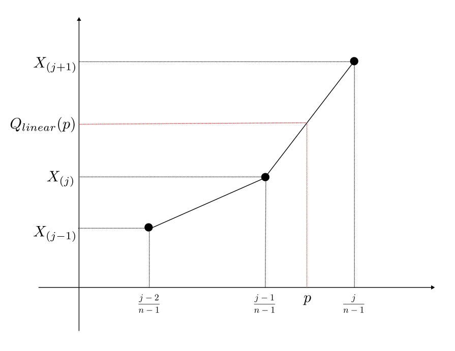
$0<p<1$ とする。
linear の $p$ 分位数 $Q_{linear}(p)$ は以下である。
$$\begin{array}{}\text{(1)}& Q_{linear}(p)=(n-1)(X_{(j+1)}–X_{(j)})p+j{X}_{(j)}+(1-j)X_{(j+1)}\end{array}$$
ただし、
$$\begin{array}{}\text{(2)}& \frac{j–1}{n–1}\le p<\frac{j}{n–1}\end{array}$$

例

イントロダクションで出した例

data = [26, 12, 30, 20, 35, 25, 1, 37, 15, 13, 9]

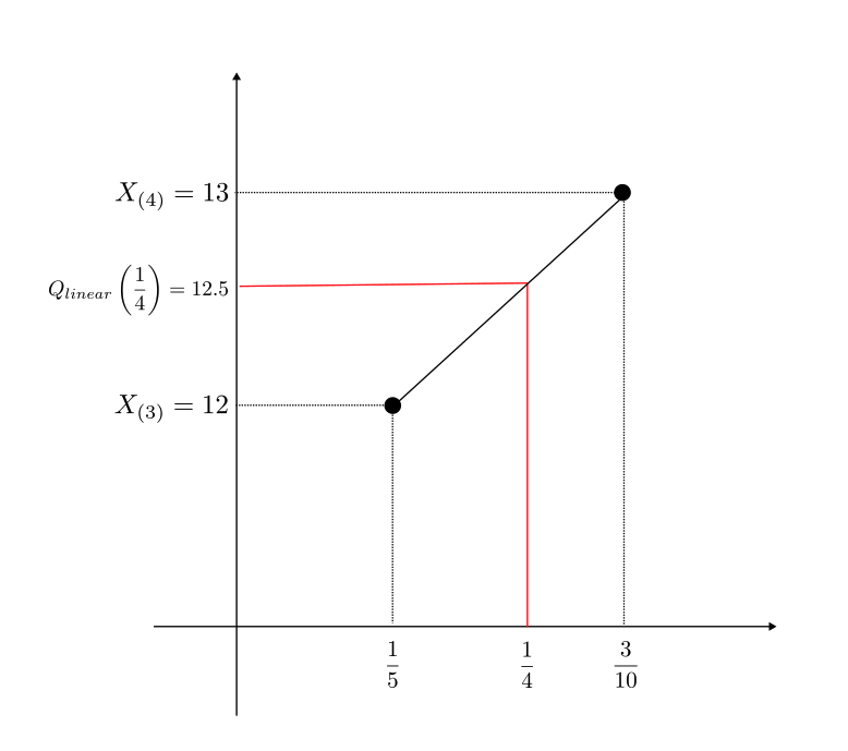
を使って、第一四分位数 $Q_{linear}(1/4)$ を求めてみる。data を昇順に並べ替えると、

[1, 9, 12, 13, 15, 20, 25, 26, 30, 35, 37]

である。まず、$(\text{2})$ から $j$ を決める。$n=11,p=1/4$ より、
$$\frac{j–1}{10}\le \frac{1}{4}<\frac{j}{10}\iff \frac{5}{2}<j\le \frac{7}{2}$$
となるので、$j=3$。よって、$X_{(3)}=12,X_{(4)}=13$ なので $(\text{1})$より、
$$Q_{linear}\left(\frac{1}{4}\right)=10(X_{(4)}–X_{(3)})\cdot \frac{1}{4}+3X_{(3)}–2X_{(4)}=12.5$$
となる。

weibullの場合

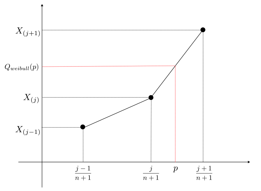
weibull の $p$ 分位数 $Q_{weibull}(p)$ は以下である。
$$\begin{array}{}\text{(3)}& Q_{weibull}(p)=(n+1)(X_{(j+1)}–X_{(j)})p+(j+1)X_{(j)}-j{X}_{(j+1)}\end{array}$$
ただし、
$$\begin{array}{}\text{(4)}& \frac{j}{n+1}\le p<\frac{j+1}{n+1}\end{array}$$

例

data = [26, 12, 30, 20, 35, 25, 1, 37, 15, 13, 9]

とし、昇順に整理すると、

[1, 9, 12, 13, 15, 20, 25, 26, 30, 35, 37]

である。$p=1/4$ とすると、$(\text{4})$ より
$$\frac{j}{12}\le \frac{1}{4}<\frac{j+1}{12}\iff 2<j\le 3$$
なので、$j=3$。

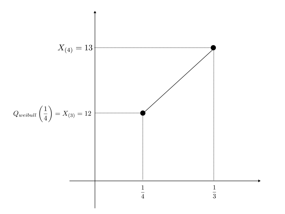
よって $X_{(3)}=12,X_{(4)}=13$ なので、$(\text{3})$ より、
$$Q_{weibull}\left(\frac{1}{4}\right)=12(X_{(4)}–X_{(3)})\cdot \frac{1}{4}+4X_{(3)}–3X_{(4)}=12$$

補足

あまり使うことはないだろうが、numpy.percentileのweibull、statistics.quantileのexclusiveでは $p<1/(n+1)$ のとき $j<1$ 、そして $p>n/(n+1)$ のとき $j>n$ となる。この場合、numpy.percentileのweibullとstatistics.quantileのexclusiveは結果が異なるようだ。

例えば、

data = [26, 12, 30, 20, 35, 25, 1, 37, 15, 13, 9]

としたとき、

import statistics
import numpy as np

data = [26, 12, 30, 20, 35, 25, 1, 37, 15, 13, 9]

# 0.01分位数
print(np.percentile(data, 1, method='weibull')) # 結果：1.0
print(statistics.quantiles(data, n=100)[0]) # 結果：-6.04

# 0.99分位数
print(np.percentile(data, 99, method='weibull')) # 結果：37.0
print(statistics.quantiles(data, n=100)[98]) # 結果：38.76

となる。

np.percentile に関しては、

$p<1/(n+1)$ のとき、$Q(p)=X_{(1)}$ $p>n/(n+1)$ のとき、$Q(p)=X_{(n)}$

となることが以下から推測できる。

import matplotlib.pyplot as plt
import numpy as np

# 座標描画用の関数
def plot_cordinate(x, y, color):
    plt.plot(x, y, marker='.', color=color)
    plt.hlines(y, 0, x, "m", linestyle=":", color=color)
    plt.vlines(x, 0, y, "m", linestyle=":", color=color)
    plt.annotate(x, xy=(x, 0), xytext=(x, -1.5), ha='center', color=color)
    plt.annotate(y, xy=(0, y), xytext=(-1, y), ha='center', color=color)

data = [26, 12, 30, 20, 35, 25, 1, 37, 15, 13, 9]
# data を昇順に並べ変える
sorted_data = sorted(data)

# j=1 のときの座標を設定
x1 = 8.3 # p = 1/12
y1 = sorted_data[0] # X_(1)

# j=11 のときの座標を設定
x11 = 91.6 # p = 11/12
y11 = sorted_data[10] # X_(11)

# dataに対してpパーセンタイルを描画
p = np.linspace(0, 100, 6001)
plt.xlim(0,100)
plt.ylim(0,40)
plt.plot(p, np.percentile(data, p, method='weibull'), color='b')

# X_(1)とX_(11)の座標を描画
plot_cordinate(x1, y1, color='r')
plot_cordinate(x11, y11, color='g')

plt.show()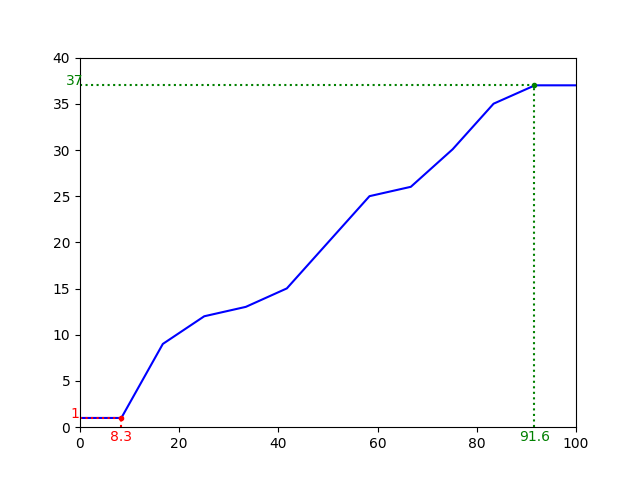

statistics.quantiles は

$p<1/(n+1)$ のとき、$Q(p)$ は点 $(1/(n+1),X_{(1)})$ と $(2/(n+1),X_{(2)})$ を通る直線上、
$p>n/(n+1)$ のとき、$Q(p)$ は点 $((n-1)/(n+1),X_{(n-1)})$ と $(n/(n+1),X_{(n)})$ を通る直線上、

となることが以下から推測できる

import matplotlib.pyplot as plt
import numpy as np
import statistics

# 座標描画用の関数
def plot_cordinate(x, y, color):
    plt.plot(x, y, marker='.', color=color)
    plt.hlines(y, 0, x, "m", linestyle=":", color=color)
    plt.vlines(x, 0, y, "m", linestyle=":", color=color)
    plt.annotate(x, xy=(x, 0), xytext=(x, -1.5), ha='center', color=color)
    plt.annotate(y, xy=(0, y), xytext=(-1, y), ha='center', color=color)

# 2点を通る直線の描画の関数
def plot_line(x1, y1, x2, y2, color):
    t = np.linspace(0,100,1000)
    m = (y1 - y2)/(x1 - x2)
    y = (m * (t - x1)) + y1
    plt.plot(t, y, linestyle='--', color=color)

data = [26, 12, 30, 20, 35, 25, 1, 37, 15, 13, 9]
# data を昇順に並べ変える
sorted_data = sorted(data)

# j=1 のときの座標を設定
x1 = 8.3 # p = 1/12
y1 = sorted_data[0] # X_(1)

# j=2 のときの座標を設定
x2 = 16.6 # p = 2/12
y2 = sorted_data[1] # X_(2)

# j=10 のときの座標を設定
x10 = 83.3 # p = 10/12
y10 = sorted_data[9] # X_(10)

# j=11 のときの座標を設定
x11 = 91.6 # p = 11/12
y11 = sorted_data[10] # X_(11)

# dataに対してpパーセンタイル(statistics.quantiles)を描画
p = [i for i in range(1, 100)]
plt.xlim(0,100)
plt.ylim(0,40)
plt.plot(p, statistics.quantiles(data, n=100), color='b')

# X_(1), X_(2), X_(10), X_(11)の座標を描画
plot_cordinate(x1, y1, color='r')
plot_cordinate(x2, y2, color='r')
plot_cordinate(x10, y10, color='g')
plot_cordinate(x11, y11, color='g')

# X_(1)とX_(2)を通る直線
plot_line(x1, y1, x2, y2, color='c')
# X_(10)とX_(11)を通る直線
plot_line(x10, y10, x11, y11, color='m')

plt.show()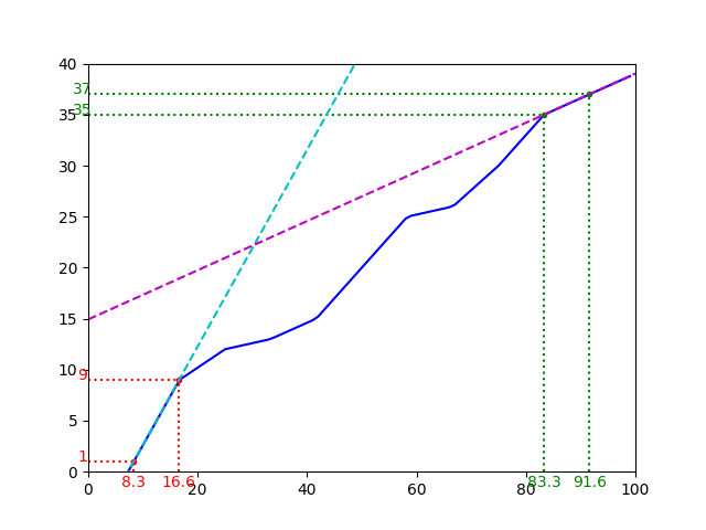

実際、$p=1/100$ で計算をしてみると、
$$\frac{j}{12}\le p<\frac{j+1}{12}$$
を満たす $j$ は
$$-\frac{88}{100}<j\le \frac{12}{100}$$
となるため、$j<1$である。$(1/12,X_{(1)})$ と $(2/12,X_{(2)})$ を通る直線の式は
$$Q(p)=96p-7$$
である。よって、$Q(1/100)=-6.04$ となることが確認できた。

参考

1. numpy.percentile — NumPy v2.0 Manual ↩︎
2. R. J. Hyndman and Y. Fan, “Sample quantiles in statistical packages,” The American Statistician, 50(4), pp. 361-365, 1996 ↩︎
3. statistics — 数学的統計関数 — Python 3.12.4 ドキュメント ↩︎